HDR Composition with PixInsight

As I anticipated in my previous tutorial, I’m going to explain one easy way to generate an HDR composition with the HDRComposition tool in PixInsight.

The data is the same I used in my previous article, plus some color data to make it “pretty”:

• Luminance: 6×5 minutes + 6x 30 seconds (33 minutes)
• RGB: 3×3 minutes each channel, binned 2×2 (27 minutes)

The two luminance sets is where we’ll be doing the HDR composition. As I also mention in my last article, this is clearly NOT high quality data. I only spent about one hour capturing all the data (both luminance sets and all the RGB data) in the middle of one imaging session, just for the purpose of writing these articles.

Of course, before we can integrate the two luminance images, all the subframes for each image need to be registered/calibrated/stacked, and once we have the two master luminance images, we should remove gradients, and register them so they align nicely. The calibration/stacking process can be done with the ImageCalibration and ImageIntegration modules in PixInsight, the registration can easily be done with the StarAlignment tool, and the gradient removal (don’t forget to crop “bad” edges first, due to dithering or misalignment) with the DBE tool.

Now that we have our two master luminance images nicely aligned, let’s get to the bottom of it. HDRComposition works really well with linear images. In fact, if you feed it linear images, it will also return a linear image – a very useful feature, as you can create the HDR composition and then start processing the image as if the already composed HDR image is what came out of your calibration steps. The first step then, once we have our set of images with different exposures nicely registered (just two in this example), is to add them to the list of Input Images:

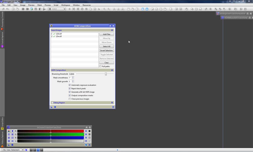
With that done, we simply apply (click on the round blue sphere), and we’re done creating the HDR composition. Well, not exactly, but almost. Considering all we’ve done is to open the HDRComposition tool, feed it the files and click “Apply”, that’s pretty amazing!

You could tweak the parameters, but really, the only things to adjust would be the parameters that define the mask creation: threshold, smoothness and growth, and as we shall see, the default values already work pretty well.

Of course, since we’ve integrated two linear images, our resulting image is also linear, which can be very handy if we would like to do some processes that work much better with linear images, such as deconvolution, etc. Regardless, being still a linear image, it appears really dark in our screen.

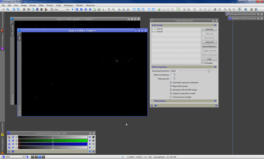
Now, being this such marginal data, the SNR of this image doesn’t grant for a successful deconvolution. We can examine the noise with PixInsight in different ways, but in this case, a simple histogram stretch (or by using the ScreenTransferFunction) is already good enough to “see” it… Therefore, we will skip the deconvolution and just do a basic histogram stretch, so we can see what’s in there:

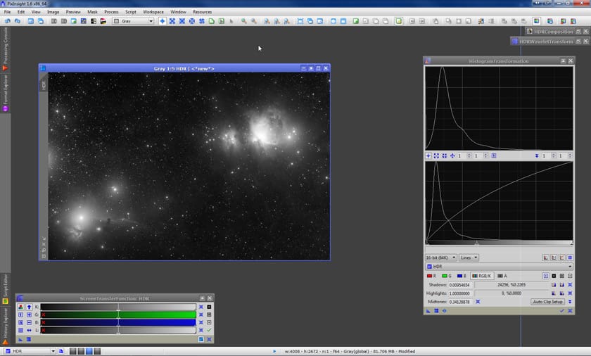
Horror! The core of M42 is, again, saturated!! Didn’t we just do the HDRComposition to avoid this very problem??

Not so fast… The HDRComposition tool has actually created a 64 bit float image (we can change that, but it’s the default and as you should remember, we used the default values). That’s a dynamic range so huge – we’re talking about 180,000,000,000,000,000,000 (if I’ve got this right) possible discrete values! – that it’s almost impossible to comprehend (some might argue it’s so huge it’s unnecessary), and definitely, quite hard to represent on a monitor that likely cannot represent data at a depth larger than 8 bit (if this last sentence confuses you, please do a search on the net to find how monitors handle color depth – discussing that here is clearly out of the scope of this article). So the data is actually there, it’s just that the dynamic range of the image is defined in such a large array, our screen cannot make up the difference between values that are “relatively close” – that is, unless we work on it a bit more.

The HDRWT tool (HDR Wavelets Transform) comes to the rescue! What the HDRWT tool does is applying dynamic range compression on a multi-scale fashion, by applying it only to specific structures at a selectable scale, leaving untouched the data at other scales.

So, again using the default parameters but of the HDRWT tool instead (it just so happens that they work really well for this image), we apply it to the image. Now, the little details in the core of M42 finally become visible (don’t worry if it’s hard to see in the screenshot below, we’ll zoom in later):

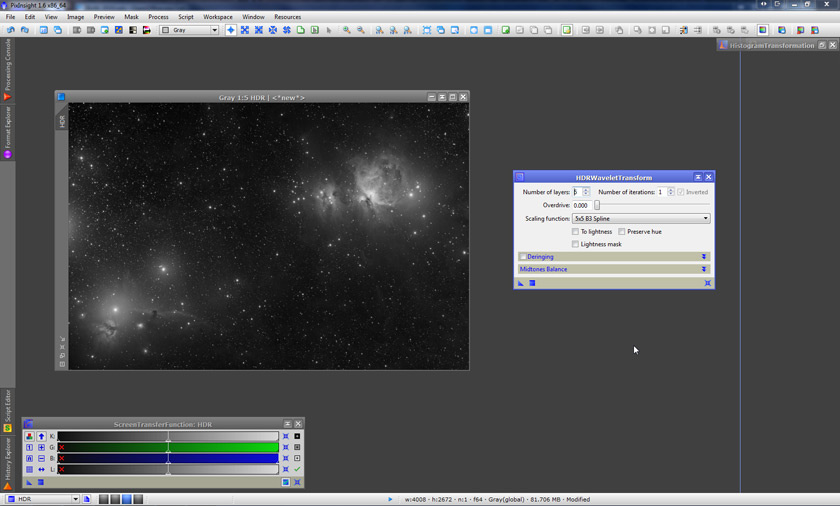
This actually puts an end to what the actual HDR composition would be. Yup, we’re done with that. There’s really nothing more to it.

Notice how the actual HDR composition was made by three incredibly simple steps:

• Selecting the two images (or as many as we have) we want to combine and applying the default parameters of the HDRComposition.
• Doing a basic histogram stretch.
• Applying the default parameters of the HDRWT tool.

If we were to compare this with the myriad of possible scenarios one would need to preview if we were using HDR-specific programs such as Photomatix, or the rather unnerving tweaking we might be doing if we were using the “Merge to HDR” tool in Photoshop, or if you were to use the “old trick” of actually doing things manually, having to layer up the two (or three or four) images, making selections, feathering them (or painting a blurred mask), fixing/touching-up edge transitions between the frames, setting the blending option and readjusting the histogram (levels) to make things match nicely… you can see how much we have simplified the process, yet obtained a pretty good result!

Why would you want to do it any other way? 😉

Once we’re reached this stage, we can try to improve the results even more, depending on our particular goals. We’re going to do this by doing a new histogram stretch, then applying the HDRWT tool once again. Here’s our image after the histogram stretch:

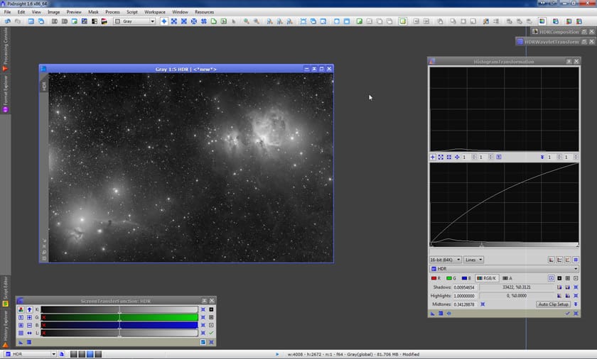
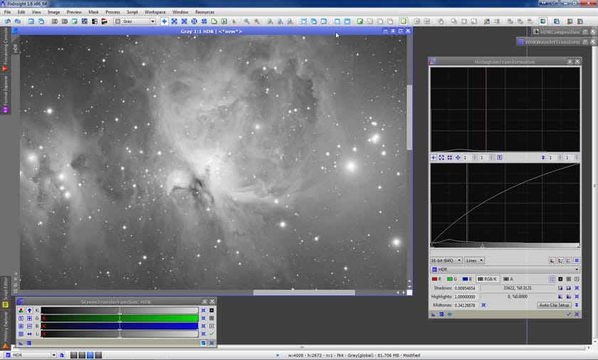
Now, let’s zoom in on the core of M42 to better see here what’s going on (of course, if you were doing this processing session, you could zoom in and out anytime). Here we can see that the core is fairly well resolved. Some people like it this way: bright “as it should be” they’d say. And you can’t argue that! (NOTE: there’s some posterization in the screen-shot below – the detail in the core actually showed up nicely on my screen).

So yeah… We could be very happy with that, but let’s go for an even more dramatic look by compressing the dynamic range once again, multi-scale style, with the HDRWT tool. We could try selecting a smaller number of layers for an even more dramatic look, but the default parameters continue to produce a very nice result, and since we want to keep the processing simple, that’s what we’ll do, and use the default parameters again. This is what we get:

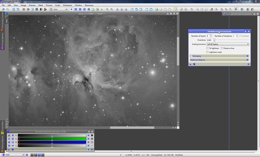
You may or may not like this result more than the previous one. Again, personal style, preferences and goals are what dictate our steps at this point, now that we have resolved the dynamic range problem.

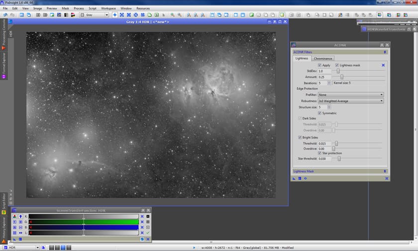
This is a good time to apply some noise reduction. We could have also done it earlier, before applying the last HDRWT. A quick noise analysis tells us that noise seems to be strong at small and very small scales, so we would apply the ACDNR tool first attacking the very small scale noise (StdDev value of 1.0), then a second pass to go for the rest, say with a StdDev value of 3.0, and then, why not, readjusting the histogram once again if we like.

Although the exercise of solving the HDR composition was already covered in the very first section, since we’ve gone this far, let’s just go and complete the image, adding some pretty colors to it.

For this purpose, I also acquired some very marginal color data but that it should suffice for this example. The data is just 3 subexposures of 3 minutes each, for each color channel (R, G and B), all binned 2×2.

I’m going to skip the step-by-step details in preparing the RGB image, but just for the record, this is what was done:

• StarAlignment, registering all three master R, G and B to the L.
• PixelMath, to combine R, G and B into a single RGB color image.
• DBE, to remove gradients.
• BackgroundNeutralization and ColorCalibration, to balance the color.
• Histogram stretch, to bring all the signal to a visible range.
• Curves Saturation, to give a bit of a punch to the color.
• SCNR, to remove green casts.

After all this was done, we end up with the gray-scale image we have been working on so far, and a nice color image. We’re now ready to do the LRGB integration:

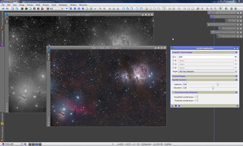
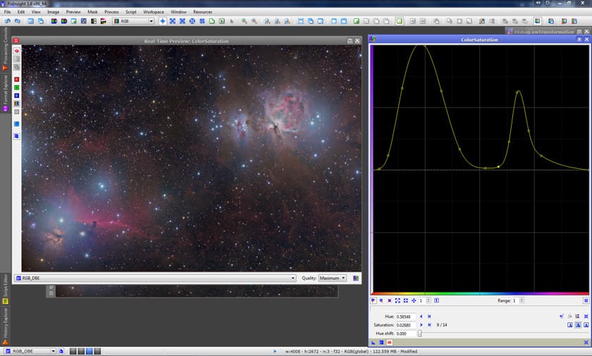
Although PixInsight offers a nice tool to adjust the lightness prior to integrate it with color data (LinearFit), in this case, the difference between both images is rather large, so I opted for skipping the LinearFit step, and manually adjust the Lightness parameter in the LRGBCombination tool. With that done and the LRGB already combined, I added a bit of a gradual saturation with the ColorSaturation tool:

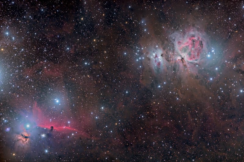
We’re almost done. The image looks very nice – especially considering how marginal the data is – but my personal taste tells me that I would rather it to have a bit more contrast. To do that, I use the DarkStructureEnhance script, along with another histogram adjustment, and with that done, I call it a day. Here’s the image, reduced in size so that it fits in this page:

And here’s a closeup of the core of M42 at the original scale:

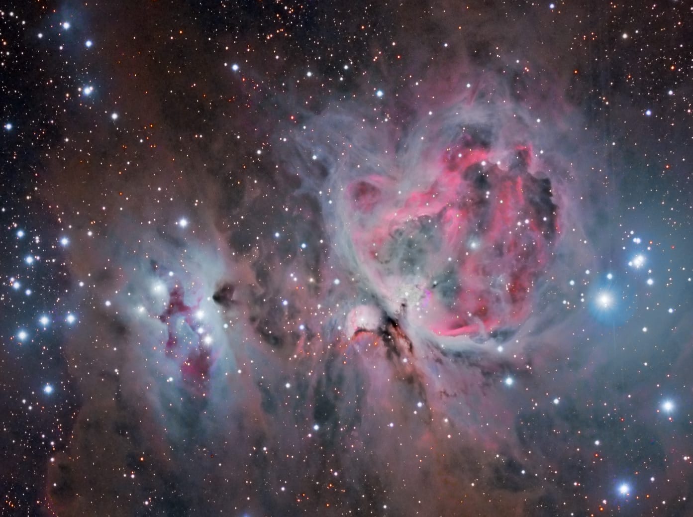
As stated earlier, this is rather marginal data, so don’t expect Hubble quality here! And of course, the resolution isn’t astonishing either because I used a FSQ106EDX telescope with a focal reducer (385mm focal length) and a STL11000, which combined, give an approximate resolution of 4.8 arcsec/pixel. Then again, the purpose of this article is not to produce a great image, but to highlight how easy it is to deal with this particular high dynamic range problem with the HDRComposition tool in PixInsight.

If you’ve been dealing with this problem by using the “old trick” of layering the images and “uncovering” one over the other via lasso selections or painted masks, I don’t know if this brief article will persuade you to try doing it differently next time, but at the very least, if you decide to stick to the “old ways”, I hope you at least remember that, well, there is a much much easier way 😉

Hope you liked it!