Removing gradients while preserving very faint background details

Gradients are often unavoidable, and they get worst the wider your field of view is. Of course, incredibly dark skies are a great help, but we don’t always have that luxury.
The strategy you choose to deal with gradients will depend on the image, how severe the gradients are, and your goals. This tutorial shows you how I deal with gradients with images that also contain very faint details in the background that I want to preserve.

Many people attack gradients somewhere in the middle of the processing of an image. While the results obtained by doing this can be ok, my experience is that it’s a lot better to deal with the gradients at the very beginning.

There are many reasons why dealing with gradients in the middle of the processing is just not a good idea: stretching an image with gradients is not desirable because our histogram isn’t true to the data we want to process – the histogram is including the gradient data, which means we’re looking at a histogram that is not a good representation of our data, and why would we want to carry the gradient data with us as we process the image and deal with it “later”? Also, color-balancing an image with gradients can be misleading, so again, ideally we want the gradients corrected before we color-balance our image, something that is better to do when the image is still linear – which also means our gradient corrections must not break the linearity of our image, they have to be done early in the process, etc. In short, gradients have been added to our image and they’re unwanted, so before processing our image we should get rid of them first, and once that’s done, proceeded as “usual”.

The most effective way of removing gradients (other than perhaps super-flats?) is by creating a background model defining the gradient and subtracting it from our image. We subtract it because gradients are an additive effect. By doing this, we can remove the gradients and be left with an image that is still in linear form, so we can then start processing it just like we would with any image – but without gradients!

The tutorial is based on a set of luminance from an image of M10, M12 and the galactic cirrus that I captured many years ago.

The captured data was of Ok quality, but as you will see, it wasn’t free of gradients. The master file was generated from 7 subexposures of 15 minutes each at -20C temperature, with a SBIG STL11k camera and a Takahashi FSQ106EDX telescope with the 0.7x reducer. The data was captured at DeepSky Ranch, California, between 1:45am and 3:30am on May 6th, 2010.

The goal in this session is to remove the gradients from the luminance, but at the same time trying to preserve some very VERY dim galactic cirrus that populates that area.

We skip the process of calibrating and registering the 7 subframes. This means we already have a “master” luminance file. We open it in PixInsight:

As usual with most astroimages, there isn’t much to see.
We want to see what’s in there, so we use the “Auto” function from the ScreenTransferFunction tool (STF from now on) to perform a strong “screen stretch”, that is, a strong stretch of the image as presented on the screen but without actually modifying any data in the image.

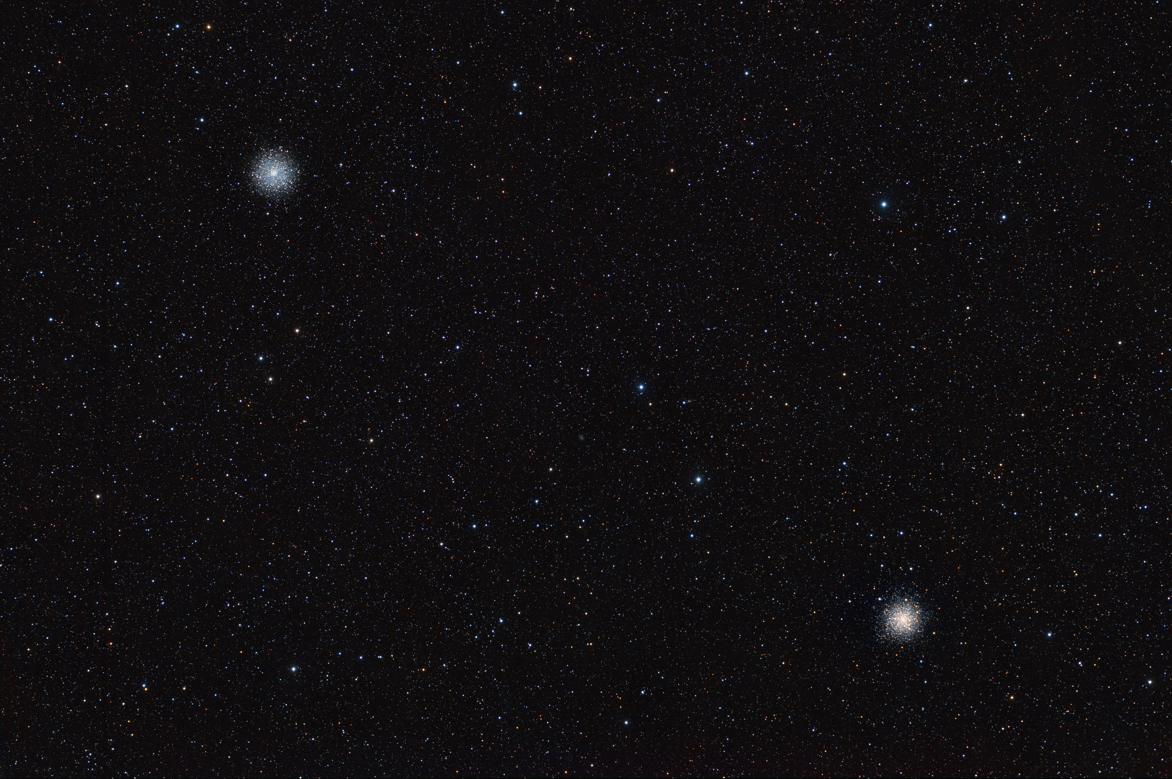
Now we can see what’s really there, and the most noticeable thing (besides a “bad column” that wasn’t corrected during calibration) is a gradient that presents our image rather bright on the left area, and much darker on the right. Our two globular clusters show nice and clear, which is nice.

If we pay very close attention, we also notice that there is in fact some data of the galactic cirrus in the image. We can tell the galactic cirrus from the gradient, because the gradient is a uniform and gradual effect across the image, but we can also see some structural differences. Yes, they’re hard to see, but with some experience (and by looking at the actual image, not at a reduced screenshot) is quite noticeable. One thing is sure, we won’t be able to do anything with that galactic cirrus unless we get rid of the gradient, and fast!

The first thing I do to create an acceptable background model is to create a duplicate of the image, and apply a non-linear histogram stretch. I do this because it will then be easier to place the samples used to create a background model based on this gradient.

Our gradient is back, indeed. In this histogram stretch we can also better see some of the galactic cirrus data that we do NOT want to remove.

Now we use the DynamicBackgroundExtraction tool (DBE from now own) to construct the background model.

Although I am not going to use the DBE symmetry function, I like to set the symmetry point at a place that seems to make sense to me, all the way to the right of the image in this case.

VERY IMPORTANT: When placing the samples that later will be used to create the background model, first I will place just a few of them, at an average of perhaps just 5-8 across. The reason is twofold. First, we’re trying to model a gradient, and gradients are usually very smooth and gradual. If we were to place many samples, our model will start not to be as smooth and gradual as the gradient, as I will show you in a minute. The other reason is that we want to preserve the very subtle differences in the galactic cirrus data in the background, and we definitely do not want the samples to catch these differences.

In the screenshot above you can (barely) see the sample points in cyan blue. Later you’ll be able to see them much better, so I’ll talk about that then.

The next step is to SAVE this process as a “Process Icon”. The reason is, we do not want to apply the DBE to this non-linear image. We have stretched this image to get a better feel of where the samples should go. By saving the process, we can then apply it to our real “good” image later.

Notice in the screenshot above the little icon next to the mouse cursor. We’ve created this process icon by dragging the “blue triangle” at the bottom-left of the DBE dialog over the workspace.

We can now close the DBE dialog and the stretched image. After doing that, we double-click on the process icon, and we “magically” apply to our “good” image the parameters we just defined earlier:

Here is when I can better show you where I’ve placed my samples. Notice I first auto-generated about 6 samples per row (equal spacing vertically) and then I’ve placed a few samples manually on the left area, where I noticed there was a very “short” darkening gradient, that our model background wouldn’t pick unless we also set a few more samples there. Generally, in order to protect the very faint background structures, we should do an even more careful placement of the samples across the image, but as we shall see, even a more general sample placement can yield good results.

With that done, we’re ready to apply the DBE. Notice (if you can read it!) that I have selected “Subtraction” as the correction formula. As I mentioned earlier, gradients are of additive nature, so in order to correct them, we must subtract the background model, rather than dividing it (which is what we’d do if we were dealing with vignetting, for example).

And here’s our corrected image after subtracting the background model created by the DBE process:

Not much to see, right? Let’s now apply a STF to both, our corrected image and the background model. This allows us to see whether the gradient has been successfully corrected as well as the shape of the background model we’ve used:

On the left you see the background model. Notice it’s a smooth and gradual model, which is exactly what we wanted. If we were looking for complete perfection, we do notice that there’s a few areas in the model that don’t seem to be “just gradient corrections”. In that case we would go back to the DBE tool, readjust the position of our samples, perhaps also readjusting some of the modeling parameters, using as a guide the background model we just created – which “tells” us where it didn’t do a good job.

On the right you see the corrected image (with a very strong STF stretch). We do notice the background is not perfectly flat. Did we fail? Nope, that’s the signal from the galactic cirrus! Other than that, we can tell the gradient is pretty much gone.

We disable the STF and our image is ready to be processed. Just as when we started but without the gradient:

Although we are confident that the uneven background signal we saw in the STF’ed image after applying our background model is not the result of gradients, in part because we were able to see that the differences in background brightness of the “screen-stretched” image do not correspond with the subtle differences we notice in our background model, a reassuring check would be to compare a quick non-linear stretch of our image with the same area from the IRAS survey, Here’s our image:

And here’s the same area from the IRAS survey:

Obviously our image does not offer the same level of detail – in some cases it might, once processed, but certainly not at this point where all we’re doing to our image is just a screen stretch – but we can see that the background areas that appear to be darker in our image roughly match the darker areas in the IRAS image. To get an even closer picture, we can apply some multi-scale processing techniques (MS) to our image so we can bring out even more clearly the background signal – for this purpose we have also applied some strong histogram adjustments (HS) over-highlighting bright areas and over-darkening darker background areas:

As I think it’s clear, our bright background structures match pretty well with the structures from the IRAS image. Of course they do NOT match exactly, that’s why when making that assesment, we must consider a couple of things:

• We’ve just collected 7×15 minutes subexposures from a less than perfect sky, so the signal we’ve captured from the cirrus is not going to be as detailed as if we had imaged the Orion Nebula.
• The quick multi-scale process we’ve applied usually blurs the large scale structures – our purpose at this point is to identify whether bright intensities in the background we have now  more-or-less match the bright areas from the survey image, and blurred structures are ok to make that assessment. You can tell by looking at the final processed image that when processed carefully, the background structures don’t look exactly like the “quick blur” we just did.
• The resolution and quality of the image we’ve obtained from the IRAS survey is also not ideal – areas that look very dark in the image may not be really absent from galactic cirrus for example. I have seen images taken with large telescopes of parts of the sky that display a large and dense amount of galactic cirrus where the images from the IRAS survey barely show any.

And of course, what really matters for the purpose of this tutorial is that the gradients we originally had in the image have no influence in this background signal, that we have been able to remove the gradients using an appropriate workflow, and that in the process we have not destroyed faint background details.

NOTE ADDED ON 5/16/2011: Teri Smoot processed WISE IR data of this area and created a video that overlaps her results with the final image used in this tutorial. Although both sets do not match 100%, I think the results are very interesting. You can see the animation here.

When creating a background model, some people tend to define a large number of samples with the idea that the more samples we place, the more accurate the background model will be.

The problem with this approach when removing gradients is that, if our image contains subtle variations in the background NOT caused by gradients, a background modeled after many samples will catch these variations, more so if the variations are not so subtle.

For example, look what happens in this case if we generate and apply a background model that was created from a large number of samples:

At the top-left is our original image with the sample marks (yup, that’s a lot of samples!).

At the bottom-left is the background model generated. You can just tell by looking at this background model that it’s not the right model to correct a gradient – unless you believe that a gradient could have that shape!

As a result, on the left is a screen stretch of the image after we’ve applied the background sample. Not only the background details we know this image has are pretty much gone, but also we can see some darkened areas – especially around bright stars or even the two clusters – that we can tell are processing artifacts. We’ve over-corrected our background.

So although there are cases where a large number of samples is justified, be careful when dealing with gradients, and always stretch your background model to make sure that it indeed shows the shape of what you’d expect from a gradient.

As always, this tutorial takes a bit of time to read, but it really only involves four very very simple processing steps:

• We screen-stretch our image to view the gradient
• We histogram-stretch a duplicate of the image to place samples at the right places
• We create and apply the background model
• We verify that the model generated is appropriate and that our final image is properly corrected

For someone with some experience working with PixInsight, this session could be carried out in just 5 to 10 minutes.

As always, feel free to leave comments, questions, suggestions…