Star size reduction via Morphological Transformations
Intro
Every once in a while, when we are processing our data, in order to craft an image aimed at communicating or displaying something specific, we run into a “problem”: the stars in the field are so conspicuous that either distract our attention from the structures behind them, or simply don’t allow us to display clearly such structures.
When that happens, one of the solutions is what in simple terms is referred as “star size reduction”.
Reducing the size of the stars in our images may sound a bit dramatic. Some people have even declared that such procedures are a sure way to produce fake images.
The truth is that, if we are trying to produce an image of aesthetic and/or documentary value, as long as we apply this star size reduction homogeneously and following a well established criteria – that is, if we “dim” all the stars that share certain characteristics, and such reduction is homogeneously applied to all of them – what we are doing is perfectly acceptable. And while these debates often ignite endless and repetitive discussions, my aim here is not to justify these methods but to show you one way to apply them. For those of us who find these methods perfectly acceptable in order to attain the goals we have set beforehand, there’s nothing fake about applying star size reduction techniques via post-processing, and it can sometimes be an enhancement to our images, while preserving and sometimes even increasing documentary value.
Strategy
The choice we need to make is whether star size reduction is what we want for any given image, in order to achieve our goals, and if so, which type of stars need to be dimmed down: the ones that present a very large size in our image, the very dim ones, mid-sized stars…
Usually, very large stars don’t need to be reduced in size. At most, they’re creating a large glow around them, and if our goal is to show what’s behind that glow, other techniques such as dynamic range compression may be more suitable for the task.
Mid-sized stars may be a target, although most commonly, when “stars get in the way” these are small to tiny stars in fields packed with thousands of them.
This tutorial will show you one way to reduce the size of small stars. Unfortunately, I started this exercise with an image that by itself really didn’t need any star size reduction. Although this may sound counterproductive and it may not show very clearly the benefits of these techniques, the concepts utilized are perfectly acceptable and the image serves the purpose of showing how it can be done. Just for the sake of argument, at the end of the tutorial I will too present a before/after example of an image that does benefit from star size reduction techniques in order to achieve the goal of not letting the stars block what’s behind them.
The Data
The tutorial is based on a set of 4 exposures of 30 minutes each of the Andromeda galaxy, at -10C temperature, with a SBIG STL11k camera and a Takahashi FSQ106EDX telescope. The data was captured at the DARC Observatory in California, on August 28th, 2011. We will be processing this data with PixInsight v1.7.
1 – Building the Star Mask
The very first step in star size reduction via Morphological Transformations (MT for short) is to build a proper star mask. This is to avoid the MT process to actually be applied to non-starry structures. Building the mask is crucial, as it will determine what stars – and in this particular example, also what areas of the stars – will be affected.
Here’s a screen shot of part of the M31 image we’re going to be working with:
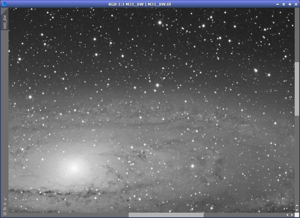
As mentioned, this image does not really call for star size reduction, but nonetheless it presents an interesting situation. We’re going to be building our star mask with PixInsight’s StarMask tool, and the brightness of the core of the galaxy and surrounding areas may produce a lack of star detection around these areas. Further, we’re attacking mid-sized to small stars in the field, but we do not want the young, blue stars that sparkle in the disk of the galaxy to be reduced at all, yet, such structures might be assumed to be what visually may appear as “small, tiny stars”.
To solve the first problem, we need to create a duplicate of our image, and “dim” the bright areas of the galaxy without dimming the stars. This can be achieved in different ways, and in this case I have chosen an idea Juan Conejero once mentioned to me: using the HDRWT tool in PixInsight, which effectively applies a dynamic range compression, to better detect stars that otherwise might be missed during the star mask creation process. Here’s the result of applying a rather aggressive HDRWT to the duplicate image:
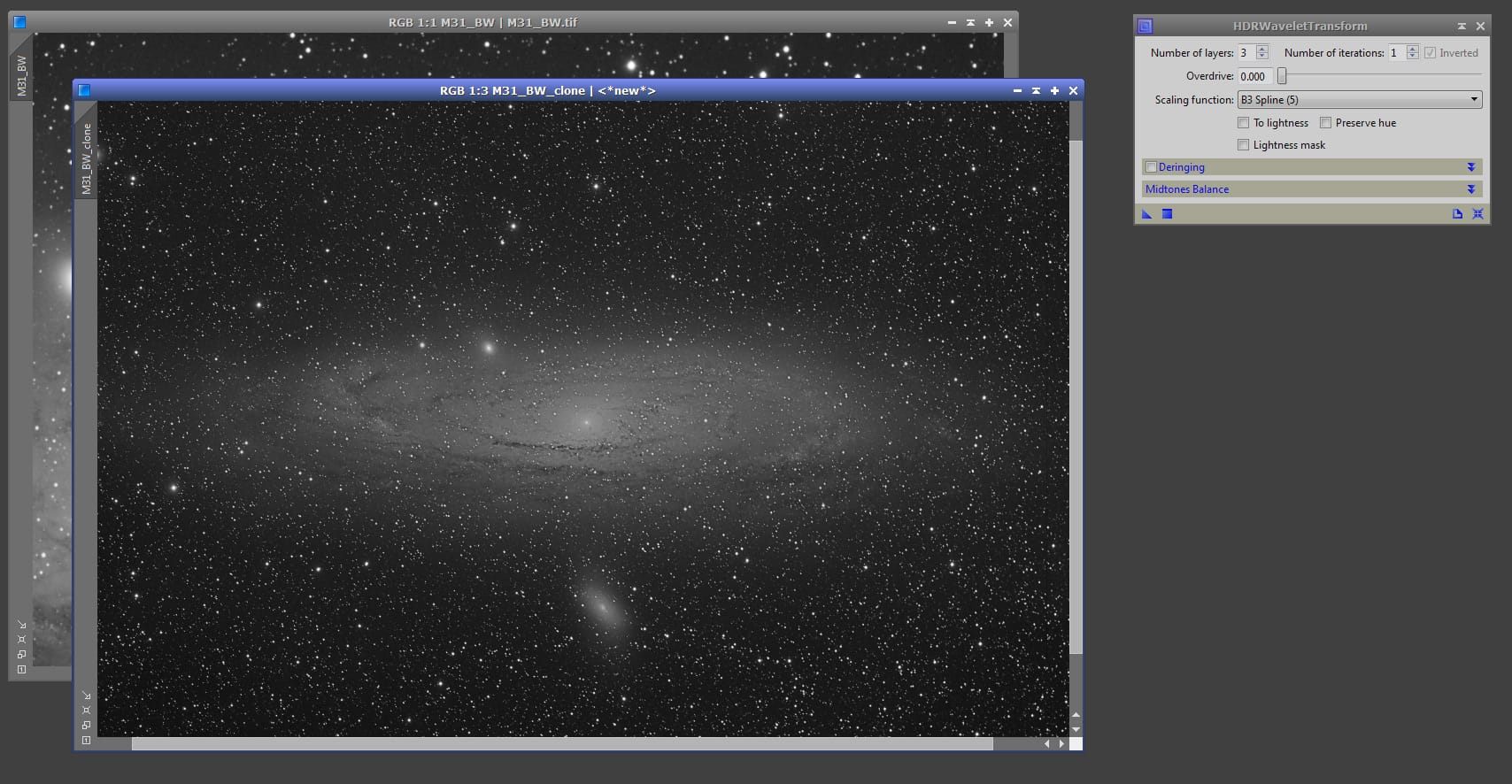
Now, the above image is better prepared to produce a suitable star mask. Depending on the case, one can apply an even more aggressive HDRWT by either increasing the number of iterations or even reapplying it several times.
It’s time to adjust all parameters in the StarMask tool to produce a star mask the way we want it in all aspects. In this case I’ve chosen the following parameters:
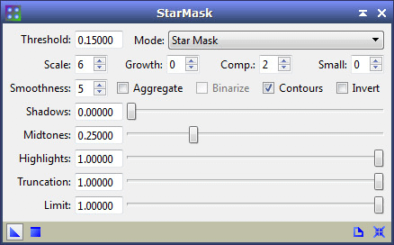
First, I’ve assigned a value of 0.15 to the Threshold parameter. The threshold parameter is meant to isolate noise from valid structures, but because a higher value will discriminate smaller structures, rising the 0.1 default a bit may help us not only avoiding noise, but also excluding the tiniest of stars in our mask.
The Scale and and Small parameters help us define the type of stars we’re after: small to mid-sized stars but not the very tiny ones. While the growth parameter is often times quite useful – it determines how much to increase the masking area – because later we’ve checked the Contours option, in order to have a well-defined contour (more on that in a bit), it’s better not to grow the masking area. Same thing with the Smoothness parameter. We don’t want to smooth out the masking areas too much, just enough, so I reduced the default value of 16 all the way to 5.
Now, the reason I’ve checked the Contour option is because, whenever possible, I want the mask to only leave unprotected the contour of the stars, which is effectively the area where the “reduction” really takes place. While going for a standard mask is often just as good, I have experienced that going for the contour exclusively gives me better results overall.
Last, note the Midtones parameter, that has a default value of 0.5, has been reduced to 0.25. This simply helps the structure detection to “stretch up” the image – equivalent to moving the midtones in the histogram to the left – which usually results in more stars being detected, and the masks being a tad thicker, since the structures are brighter after pushing the midtones to the left.
NOTE: You should not take these StarMask parameters as a cooking recipe! The StarMask tool uses a multiscale algorithm to isolate significant image structures during the structure detection phase that is strongly dependent on large-scale features of the whole image. In plain English this means that for a given set of parameters, the results you can obtain with StarMask when applied to one image, may be quite different than what you may obtain with the very same set of parameters on a different image. So the key is to understand the effects that modifying these parameter can achieve, and adjust them until the resulting mask is what you were after, or at least close enough.
Once applied, here’s the star mask we produced:
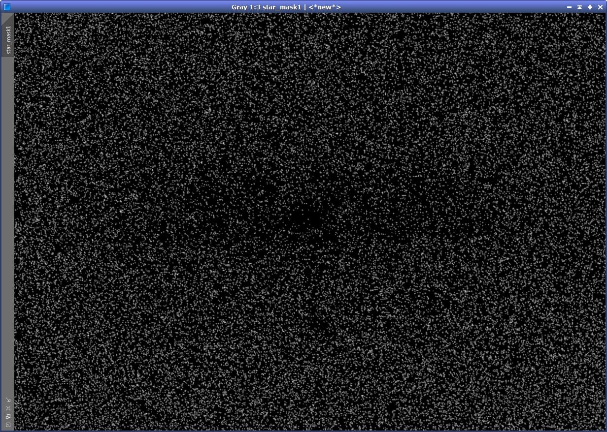
Since it’s hard to see the details in the above image, here’s a close-up at a 1:1 scale:
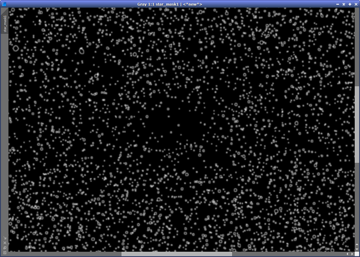
So we apply the mask and here’s how it looks (3:1 scale) when using red color as overlay to see what is being protected (red) and what’s not (transparent):
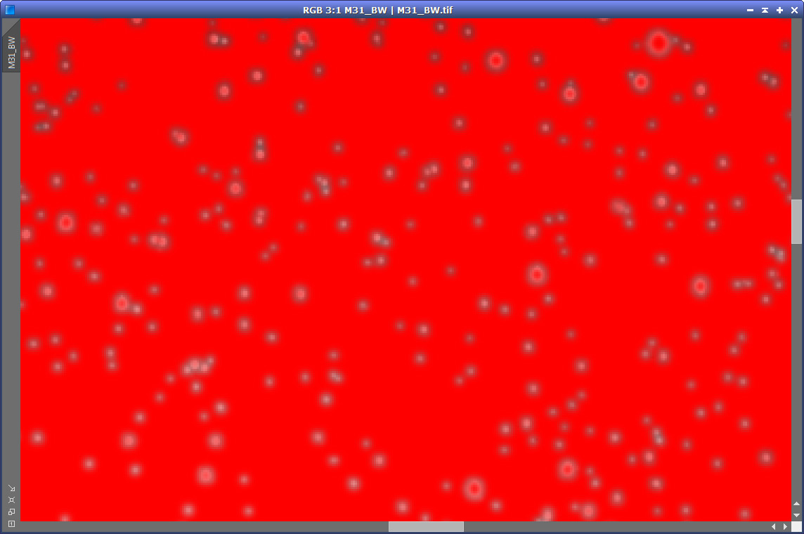
2 – Defining and applying the Morphological Transformation
With the mask in place, we now can invoke and apply the MorphologicalTransformation tool. Here’s a screen shot with the image after applying MT, and the MT dialog box displaying the parameters we used (I’ll explain them right after the image):
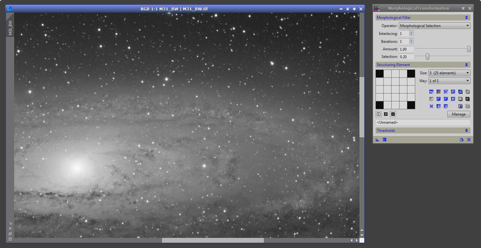
In the MT tool, first I’ve chosen the Morphological Selection operator. Most people use the Erosion operator, and it is in fact a proper option, but I like using Morphological Selection because it acts as a blend between the erosion and dilation methods, where, with the Selection parameter you can define how much erosion and how much dilation you want to apply (more erosion the closer you are to a value of 0, and more dilation as you get closer to a value of 1). And while the use of a blend of erosion and dilation in stars usually isn’t necessary – as neither are other operations that combine them, such as opening and closing – I like the smoother results that they often generate, versus applying erosion and nothing else.
Last, a round structuring element makes a lot of sense of course, and in this case I chose a 5×5 kernel size because the stars being targeted fit well within that kernel.
Once applied, our stars are now less “in your face” as they were before. As mentioned earlier, this particular image doesn’t really benefit from applying this procedure, but leaving that aside, hopefully you can see the difference.
The results we’ve obtained can be seen more clearly in this x5 zoomed-in before/after animation:
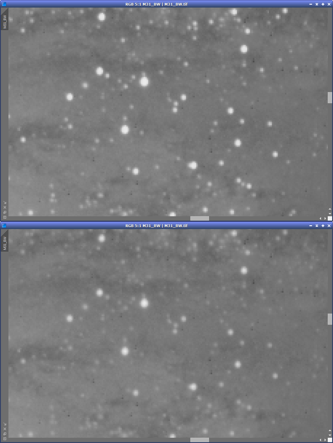
You can see that the very small stars are not nearly as discernible as they were, the small-to-midsized stars are not only “reduced” in size but also their profile is more round in appearance, and the very tiny, almost invisible stars, are untouched.
3 – Sharpening the results
We may consider that the Morphological Transformation process we’ve applied has been successful and stop right now. However, in practice, I often like to bring back some of the “life” in the stars that are now dimmer and reduced, but of course without bringing them to their previous state – otherwise I may just not do any MT at all to begin with!
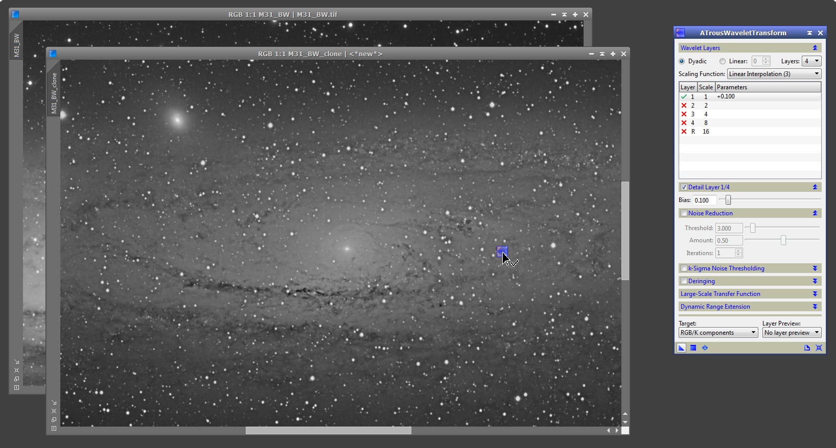
This can be achieved in several different ways, and one of such that I use quite often is by defining another star mask that protects everything but the very small scales in the image, and then use wavelets to increase a bit the bias at those scales.
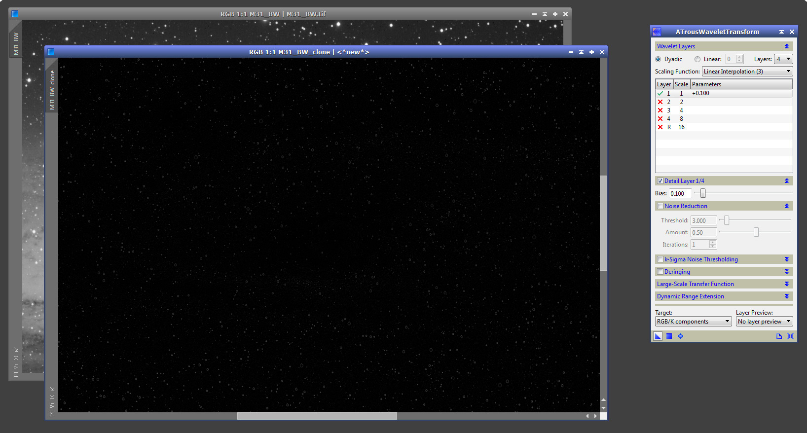
Building the mask this time is very easy. We simply use the ATrousWaveletTransform tool in PixInsight, deselect all scales except scale 1, increase the bias just a bit, and apply this to the duplicate image to which we applied the HDRWT earlier. Here’s a screen shot doing just that:
And here’s the mask we just created:
We apply the mask to our image, and then sharpen it only in those tiny “holes” defined by the mask, using the ATWT tool, by using the default values except for an increase in the bias at the smallest scale:
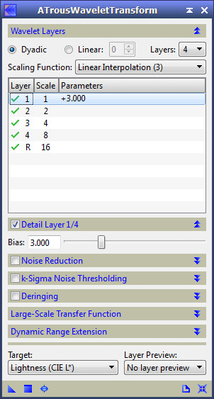
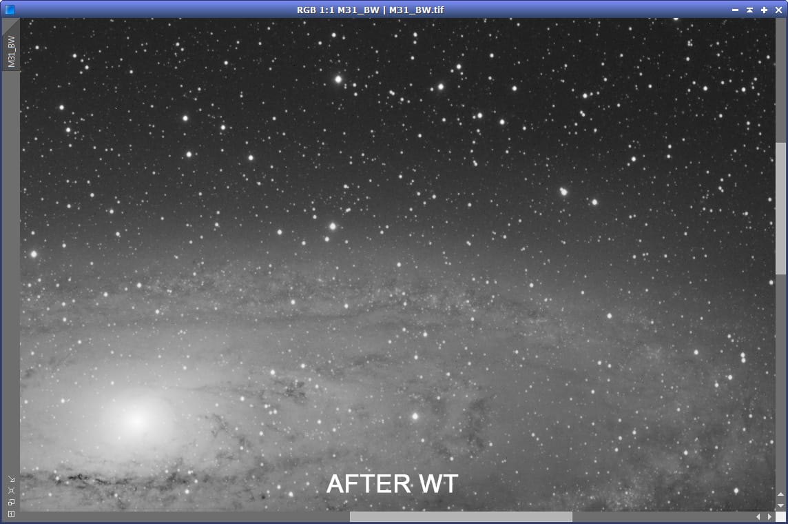
I used a bias of 3 in this case, which is A LOT!! In this case the mask was aggressive, and so the effect is greatly reduced, but you will need to dial the bias to a value you’re happy with via experimentation. And here’s the result:
4 – Before/After animations
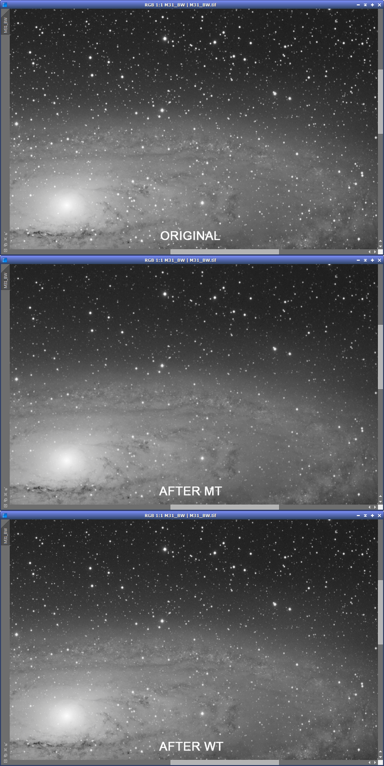
The following animation is big, but it shows the image cycling from the original version, to the version after the MT, to the version after the ATWT:
Last, here’s an animation that shows a large closeup of a single star as it was originally, and as it finally ended up after the MT and ATWT processes:
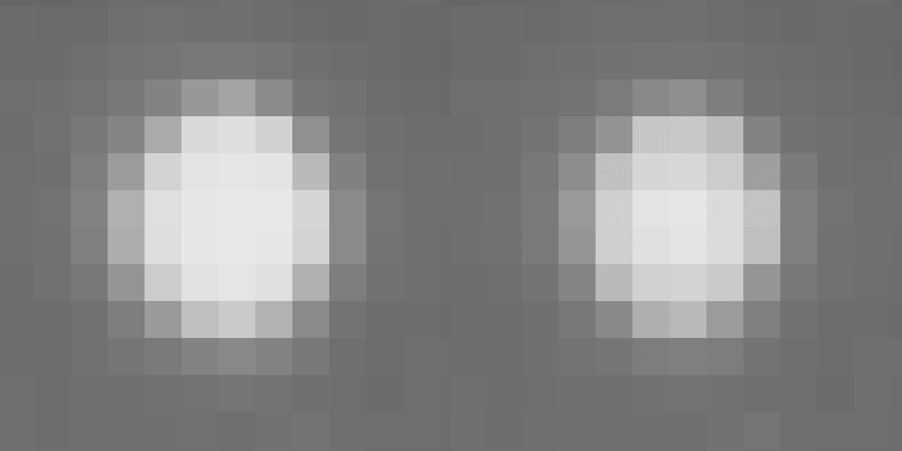
While the appearance of our image has changed considerably – ok, picture this effect on an image that was packed with stars, rather than this M31 shot – I think it’s safe to say that the data manipulation involved didn’t invent any new data around the stars. It simply “dimmed” the stars, and unlike what some people often thing of these methods, without fabricating artificial “nebula” data around them.
5 – Conclusions
If you have read all the way until here… Well.. You’ve read a lot! 😉
As it often happens, as I aim at describing each step in details (rather than just saying “do this, then that, then this, you’re done”), this tutorial may seem to be describing a rather lengthy process, but in reality it only involves a few simple steps:
- Create a star mask suitable for MT, which in this case it involved using the HDRWT and StarMask tools
- Apply MT to our image to “reduce” our stars
- Create a second star mask, this time with the ATWT tool
- Apply ATWT to “sharpen” the image a bit.
That’s all.
6 – A more suitable example
Here is a quick before/after animation of an image probably better suited for star size reduction:
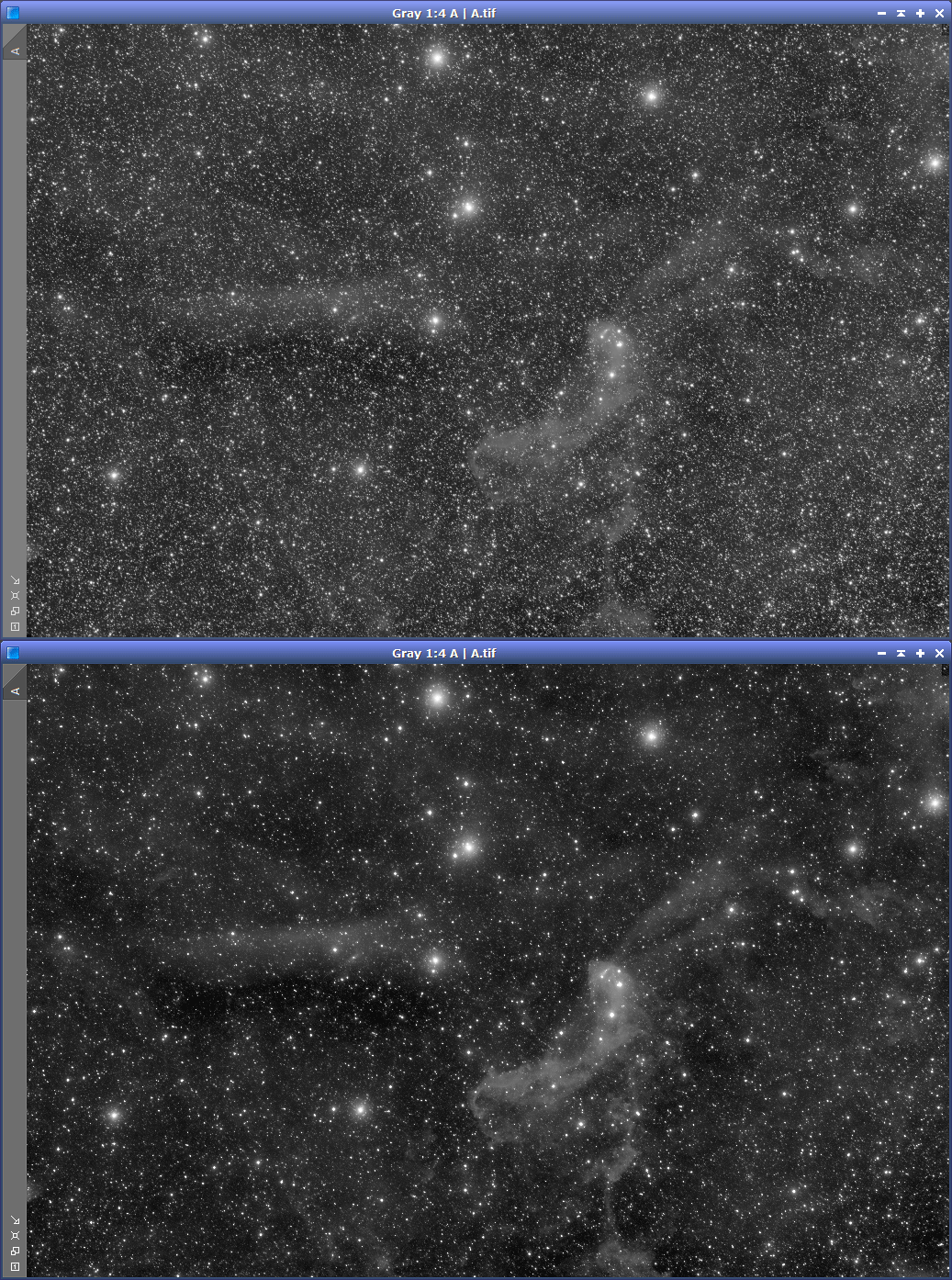
The above is an image of some very faint dust clouds in Lacerta, and it accumulated 7 hours of exposure under very dark skies (SQMs at 21.7 or above, at the zenith) with a 4″ scope at f/3.65.
There is nothing wrong with the before image. It shows a field packed with stars to the point that it’s nearly impossible to discern the faint clouds. That’s just a reality. It just happens that there are a lot of stars in that field!
However, by applying the very same “star size reduction” technique described in this tutorial, we have an image that allows us to better see the dusty structures that before were so elusive, and so we have a better visualization of the nebula. The before image tells a story, but so does the after image – and both stories are concordant with facts revealing a reality.
Not only that, after the MT procedure, we can, if we like, continue post-processing the image to even better visualize the faint clouds. The after image not only has aesthetic value, but also documentary value.
